Hierarchical Transformer Preconditioning for Interactive Physics Simulation

Carl Osborne, Minghao Guo, Crystal Owens, Wojciech Matusik

MIT CSAIL

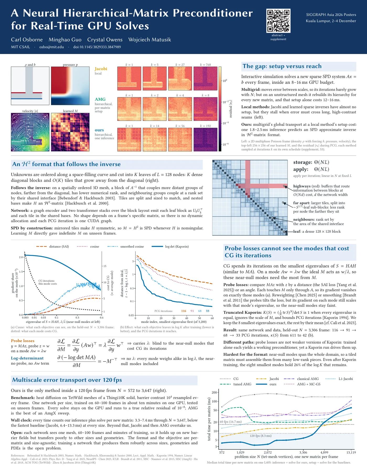
Teaser figure for the hierarchical transformer preconditioner.
Fig. 1. Teaser. Hierarchical neural preconditioning for interactive multiphase Poisson solves: weak-admissibility H-matrix prior, learned preconditioner M≈A^-1, multiscale residual transport induced by M, and 3D multiphase fluid simulation application context.

Introduction

Real-time simulation of fluids, soft bodies, and coupled multiphysics often reduces every time step to a large sparse SPD solve attacked with preconditioned conjugate gradient (PCG) (Saad 2003). The preconditioner M\!\approx\!A^{-1} is the dominant design variable. Classical choices — Jacobi, incomplete Cholesky/LU (IC/ILU), sparse approximate inverses (SPAI), and algebraic multigrid (AMG) (Lin and Moré 1999; Kolotilina and Yeremin 1993; Benzi, Meyer, and Tŭma 1996; Ruge and Stüben 1987) — excel when the matrix is reused across many solves so a heavy setup amortizes. In an interactive setting A changes every frame, so any preconditioner whose setup approaches the per-frame budget cannot amortize; IC and AMG suffer worst (Naumov et al. 2015; L. Liu et al. 2016; Yamazaki, Tomov, and Dongarra 2020).

Machine learning offers an alternative: train a neural preconditioner once and amortize the cost across frames. Graph neural networks have been the dominant choice (Y. Li et al. 2023; Häusner, Öktem, and Sjölund 2023; Chen 2024; Yang et al. 2025) because a sparse matrix has a natural graph interpretation, but the choice forces two limitations that become acute in real-time simulation. (i) GNN preconditioners typically inherit the sparsity of A, so non-adjacent interactions are either dropped or only reached through repeated graph convolutions that oversmooth local detail (Wu et al. 2019; Trifonov, Muravleva, and Oseledets 2025). (ii) The dominant operations at apply time — triangular solves on a learned IC, or two SpMVs on a learned SPAI — are bandwidth-bound and either serialize on data hazards or scatter through irregular memory.

From PCG geometry to hierarchical structure.

The ideal preconditioner is A^{-1}, which is dense even when A is sparse, so the question is what structure makes A^{-1} cheap to store and apply. In modern simulation codes the degrees of freedom are already laid out along a space-filling curve (Morton, Hilbert) or a bandwidth-reducing permutation, because the surrounding pipeline (spatial hashing, BVH, neighbor search) wants that ordering (Karras 2012; Teschner et al. 2003; Ihmsen et al. 2011). Under such orderings the nonzeros of A cluster near the diagonal and the corresponding off-diagonal blocks of A^{-1} describe long-range interactions whose numerical rank decays with separation. Hierarchical matrices (\mathcal{H}-matrices) (Hackbusch 1999; Hackbusch and Khoromskij 2002; Börm, Grasedyck, and Hackbusch 2003) exploit exactly this — a recursive block partition with dense diagonal blocks and low-rank off-diagonal blocks — and the fast multipole method (Greengard and Rokhlin 1987) factors the same prior for translation-invariant kernels. An \mathcal{H}-matrix preconditioner is architecturally an FMM-shaped operator on the assembled system, and that is the prior we hand the network.

Approach.

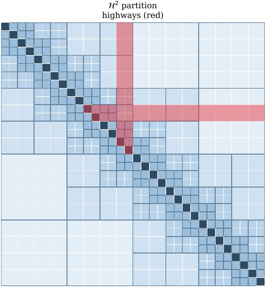
We anchor the preconditioner to a weak-admissibility \mathcal{H}-matrix partition (Hackbusch and Khoromskij 2002), computed analytically from the leaf-index geometry and reused for every frame: K\!=\!N/L dense diagonal blocks of size L\!\times\!L plus off-diagonal tiles spanning S\!\times\!S leaves with S\!=\!2^j. A two-stream transformer operates on this layout. A diagonal stream emits one factor per leaf at full rank; an off-diagonal stream emits one factor per tile at a constant coarse token count L_s\!\ll\!L regardless of S, so the rank fraction L_s/(SL) shrinks automatically with separation — exactly the bias \mathcal{H}-matrix compression calls for. To let the network route information between blocks without breaking the \Theta(N) budget, we add per-layer highway buffers (axial row/column bands plus a single global token, §4.3).

A loss with no preferred eigenvalue location.

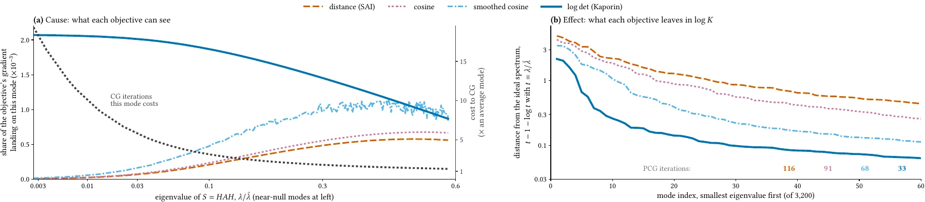
We train self-supervised with a cosine-similarity Hutchinson probe loss on the preconditioned image MA\mathbf{z}. The conceptual move over the Frobenius/SAI loss used by (Yang et al. 2025) is to replace a distance between vectors (\|\tfrac{1}{\|A\|}AM\mathbf{z}-\mathbf{z}\|_2) with a distance between subspaces (the angle between the lines spanned by \mathbf{z} and MA\mathbf{z}). This is invariant under positive rescaling of M, exactly matching PCG, which cares about the direction MA sends each probe and not the magnitude. The network is then free to cluster the spectrum of MA wherever angular alignment is easiest, with no implicit demand that the cluster live near any particular eigenvalue (Prop. 1; spectral evidence in Fig. 1). Empirically, this is not a minor objective tweak: with architecture and training split fixed, the loss swap alone accounts for a major quality gap in Table Table.

One CUDA Graph for the whole iteration.

The choices above together remove the data dependencies that normally fragment a CG iteration into separately dispatched kernels: the partition is fixed, every tile shape is the same, the apply is batched GEMMs over preallocated tensors with no triangular solves and no allocations. The whole PCG inner loop — preconditioner apply, SpMV, SAXPYs, dot reductions — records into one CUDA Graph that replays per iteration with zero CPU dispatch overhead. In our measurements this is a substantial share of the gap to classical GPU preconditioners.

Contributions.

In short: [c1] a neural preconditioner that bakes the \mathcal{H}-matrix block partition in as a structural prior with a fixed coarse rank on every off-diagonal tile, keeping total work at \Theta(N) (intro paragraph c1, §4.2); [c2] highway buffers that route information between blocks without growing the budget (§4.3); [c3] a cosine-similarity Hutchinson loss that minimizes a distance between subspaces rather than between vectors, exactly matching PCG’s scale-invariance and freeing the network to put the spectrum of MA wherever convergence is easiest (intro paragraph c3, Prop. 1 in §6.1); [c4] an allocation-free apply with no triangular solves, no data-dependent branching, no per-kernel CPU dispatch — the whole PCG inner loop captured as one CUDA Graph (intro paragraph c4, §5). Table 1 summarizes the per-iteration access pattern and throughput limit of each preconditioner family at the one step where every fixed-pattern alternative loses time on modern GPUs.

Per-iteration preconditioner application: arithmetic cost, dominant memory-access pattern, GPU throughput limit, and whether the apply admits single-CUDA-Graph capture of the PCG inner loop. \mathrm{nnz} is the nonzero count of the relevant factor. “L_s” is our fixed coarse-token count per off-diagonal tile.
Method FLOPs Memory access GPU bottleneck Graph
Jacobi O(N) stride-1 read memory bandwidth
IC (tri. solve) O(\mathrm{nnz}) wavefront-dep. SpTRSV latency / data hazards \times
Neural SPAI (Yang et al. 2025) O(\mathrm{nnz}) random gather (SpMV) memory bandwidth
AMG (V-cycle) O(N\log N) multilevel, irregular level synchronization \times
Ours O(NL_s) batched GEMM, stride-1 compute (Tensor Cores)

Related Work

Classical preconditioners.

Jacobi, incomplete Cholesky/LU, sparse approximate inverses (SPAI), and algebraic multigrid (Saad 2003; Lin and Moré 1999; Kolotilina and Yeremin 1993; Benzi, Meyer, and Tŭma 1996; Ruge and Stüben 1987; Naumov et al. 2015) are mature and remain default choices when the system is reused across many solves so a careful setup amortizes. The known GPU costs of triangular solves (L. Liu et al. 2016; Yamazaki, Tomov, and Dongarra 2020) and of V-cycle communication (Naumov et al. 2015) bite hardest in the regime we target (A changing every frame at interactive rates), which motivates the amortized neural alternative pursued here.

Learned PDE solvers and preconditioners.

Neural operators (Fourier (Z. Li et al. 2021), DeepONet (Lu et al. 2021), graph-based (Z. Li et al. 2020b, 2020a)) and physics-informed networks (Raissi, Perdikaris, and Karniadakis 2019) learn function-space mappings between coefficient and solution fields, and have been used both as surrogates and as inner preconditioners for flexible Krylov solvers (Rudikov et al. 2024); we operate one rung lower, on the assembled algebraic system. A productive line of work trains GNNs to emit a learned IC factor (Y. Li et al. 2023; Häusner, Öktem, and Sjölund 2023; Trifonov et al. 2024) or a sparse approximate inverse in factored GG^\top form using a scale-invariant Frobenius (SAI) loss (Yang et al. 2025); we compare to the latter directly in Table Table. Chen (Chen 2024) reports strong performance across SuiteSparse problems where classical IC and AMG struggle, and Trifonov et al. (Trifonov, Muravleva, and Oseledets 2025) argue that message-passing GNNs cannot approximate the non-local elimination structure of sparse triangular factors — a motivation for architectures (like ours) that route global information through explicit channels.

Hierarchical neural and matrix machinery.

A parallel line embeds FMM/\mathcal{H}-matrix structure into neural architectures (Fan et al. 2019; Z. Li et al. 2020a; Fognini, Betcke, and Cox 2025; Sittoni et al. 2026; Xu, Li, and Xi 2025; Lyu et al. 2026; Luz et al. 2020). Classical \mathcal{H}- and \mathcal{H}^2-matrix arithmetic (Hackbusch 1999; Hackbusch and Khoromskij 2002; Börm, Grasedyck, and Hackbusch 2003) provides near-linear-cost machinery for storing and applying operators with low-rank well-separated sub-blocks; HODLR variants (Hartland et al. 2023) apply the same prior to dense Hessians. The partitioning machinery is what we instantiate; the contribution lies in how the off-diagonal factors are produced and applied (§4).

Background

CG converges through the polynomial bound \|\mathbf{e}_k\|_A \;\le\; \|\mathbf{e}_0\|_A\,\min_{p\in\mathcal{P}_k,\,p(0)=1}\; \max_{\lambda\in\sigma(A)}|p(\lambda)|, so CG only sees A through how small a polynomial fixed to 1 at the origin can be made on \sigma(A). The practical consequence we lean on is that when \sigma(MA) collapses to c tight clusters away from zero, CG converges in \sim\!c iterations regardless of where on the real line those clusters sit. The preconditioning objective is therefore “cluster \sigma(MA),” not “make MA close to I,” with cluster location essentially free — the property our cosine loss exploits.

An \mathcal{H}-matrix (Hackbusch 1999; Hackbusch and Khoromskij 2002; Börm, Grasedyck, and Hackbusch 2003) represents a dense matrix as a recursive block partition: dense diagonal blocks plus off-diagonal blocks stored as low-rank factors UV^\top, with admissible rank shrinking off the diagonal because the underlying Green’s function is smooth there. We use the weak-admissibility variant (Hackbusch and Khoromskij 2002; Hartland et al. 2023), whose fewer, larger off-diagonal tiles batch well on a GPU; classical \mathcal{H}-matrix arithmetic costs O(N\log N), our learned realization runs at \Theta(N) thanks to the fixed coarse-token count in {\text{c1}}.

The training loss uses Hutchinson-style probes \mathbf{z} with \mathbb{E}[\mathbf{z}\mathbf{z}^\top]\!=\!I (Hutchinson 1989), but not as a trace estimator. The property we use is spectral whiteness: isotropy gives \mathbb{E}[(\mathbf{u}_i^\top\mathbf{z})^2]\!=\!1 for every eigenvector \mathbf{u}_i of MA, so a scalar built from (\mathbf{z},MA\mathbf{z}) weighs every eigenmode equally rather than favoring smooth or oscillatory ones — the property that makes the cosine loss of c3 a faithful global indicator of preconditioner quality.

Method

Notation and pipeline.

A\!\in\!\mathbb{R}^{N\times N} is the assembled sparse SPD system, indexed along a space-filling-curve or bandwidth-reducing ordering. The N indices are partitioned into K\!=\!N/L contiguous leaves of size L, inducing an \mathcal{H}-matrix partition of K diagonal blocks and M_{\mathcal{H}} unique weakly-admissible off-diagonal tiles (tile m spans S_m\!\times\!S_m leaves). The network is a four-stage pipeline: a physics-aware encoder, a diagonal attention stack (full per-node resolution L), an off-diagonal attention stack (coarse token count L_s\!\ll\!L, the same for every tile), and linear decoder heads. The whole network dispatches exactly two attention kernels regardless of N — one batched over leaves, one batched over tiles — which, together with the static partition, is what later lets the entire PCG inner loop run inside a single CUDA Graph. We use L\!=\!128, L_s\!=\!32, d\!=\!128, n_l\!=\!3 in every reported result.

Encoder

A two-layer MLP lifts whichever per-node features the simulator already exposes (position, velocity, density, pressure, material parameters) plus the geometric and coupling features (\Delta\mathbf{x}_{ij}, A_{ij}) for every nonzero of A to width-d node embeddings; n_{\mathrm{gcn}}\!=\!2 residual graph-convolutional layers (Kipf and Welling 2017) mix in neighborhood information using A as the message-passing weight. This is the only stage that observes individual graph edges; everything downstream operates on the block layout of the partition, decoupling cost from \mathrm{nnz}(A). Because M is neural rather than algebraic, the network can look at (\rho_i, \Delta\mathbf{x}_{ij}) directly — physical structure a fixed analytical preconditioner cannot see (full feature list in Supplementary [SX-supp:architecture]).

Diagonal and off-diagonal attention stacks

Diagonal stack. For each of the K leaves, n_l transformer layers (Z. Liu et al. 2021; Vaswani et al. 2017) with within-leaf (Swin-style) attention and edge-bias logits emit a dense factor F_k\!\in\!\mathbb{R}^{L\times L}. The corresponding diagonal block of M is the PSD outer product F_kF_k^\top.

Off-diagonal stack. For each off-diagonal tile m of size S_mL\!\times\!S_mL, node embeddings on its row- and column-strips are pooled to a fixed coarse token count L_s\!=\!L/p_{\mathrm{off}}\!\ll\!L regardless of S_m. n_l transformer layers over these L_s tokens emit a factor pair U_m,V_m\!\in\!\mathbb{R}^{L_s\times L_s}; the tile’s coarse representation is B_m\!=\!U_mV_m^\top. Because the token count is the same on every tile, the implied rank fraction L_s/(S_mL) shrinks automatically with separation — exactly the \mathcal{H}-matrix prior that distant blocks need less rank. A rank-fraction audit on real frames confirms the architecture-provided L_s/(SL) stays above what truncated SVD needs at \varepsilon\!\in\!\{10^{-3},10^{-6},10^{-9}\} in every distance class (Fig. 2; assembled-M visualization in Supplementary, Fig. [SX-supp-fig:matrices]). With S_m doubling geometrically, M_{\mathcal{H}}\!=\!O(K) unique off-diagonal tiles, and a tile-batched attention of fixed shape, the total work over the off-diagonal stack stays linear in N.

Highway connections

Within-block attention is local by construction. To let the network route information across the matrix without giving up the \Theta(N) budget, after every attention sublayer we scatter-add block-token embeddings into three buffers per transformer layer: a row-band axial buffer \mathbf{r}_{\mathrm{hw}}, a column-band axial buffer \mathbf{c}_{\mathrm{hw}}, and a single global summary token \mathbf{g}_{\mathrm{hw}}. Each token then concatenates its row, column, and global context with its own embedding before the FFN sublayer. The four channels per layer (2D intra-block, 1D row, 1D column, 0D global) cost O(Nd) scatter-gather and preserve \Theta(N) scaling. We ablate the highways in §7.3 and illustrate the per-layer connectivity in Supplementary, Fig. [SX-supp-fig:partition-and-highways]b.

Decoder, geometric picture, and complexity

Three linear decoder heads project tokens to the final factors: a leaf head emits F_k\!\in\!\mathbb{R}^{L\times L} (diagonal block F_kF_k^\top, PSD by construction); two off-diagonal heads emit U_m, V_m\!\in\!\mathbb{R}^{L_s\times L_s}; two node heads emit per-leaf bridges \tilde U_k, \tilde V_k\!\in\!\mathbb{R}^{L\times L_s} between node resolution and coarse tile resolution. A small learned per-node Jacobi gate \lambda_i adds a diagonal correction \mathrm{diag}(\boldsymbol\lambda)\mathrm{diag}(A)^{-1} that absorbs gradient early in training and decays toward zero as the structured branches take over (Supplementary [SX-supp:architecture]). In reported runs we do not explicitly enforce strict SPD and did not observe instability; if a strict guarantee is required, one can add a tiny positive diagonal shift (e.g., softplus-parameterized, as in prior learned preconditioners (Yang et al. 2025)). All factors pack into a single tensor of width P\!=\!KL^2+M_{\mathcal{H}}L_s^2+2NL_s+N that the apply consumes without ever materializing M.

Complexity and measured breakdown.

Encoder cost is O(Nd^2), diagonal stack O(n_lNLd), off-diagonal stack O(n_lNL_s^2d/L), highways O(n_lNd); total inference is \Theta(N). At N\!=\!8\,192, the subsystem profile in Table 2 shows that the two attention stacks account for 59\% of device time, while encoder + decoder remain secondary. Kernel-level profiling in Table 3 then explains why: CUTLASS Tensor-Op GEMMs (31\%) and fused attention (14\%) dominate, so the workload is primarily compute-bound on Tensor Cores rather than bandwidth-bound on sparse gathers. This directly supports the access-pattern argument in Table 1.

Subsystem breakdown of one forward pass at N\!=\!8\,192. Attention layers scale with n_l; everything else is independent of depth.
Subsystem % device time Scales with
Diagonal attention stack 36\% n_l
Off-diagonal attention stack 23\% n_l
Decoder heads 18\%
Encoder (MLP + GCN) 16\%
Layout helpers / scatter <\!4\%
Kernel-level breakdown at N\!=\!8\,192. Dominant kernels are compute-bound Tensor-Core GEMMs and fused attention; no SpMV or indexed-gather kernel appears among the top kernels.
Kernel family % device time
CUTLASS Tensor-Op GEMMs (s1688gemm, sm90_xmma, TF32) 31\%
CUTLASS fused attention (fmha_cutlassF) 14\%
Elementwise / normalization 17\%
Copies / reshapes / layout 17\%
Other 21\%

Preconditioner Application

M is never assembled. The apply consumes the packed factor tensor and produces M\mathbf{r} through three stages on preallocated buffers, with shapes fixed at solve setup by the static partition. (i) A diagonal stage applies F_k to each leaf residual \mathbf{r}_k in one batched GEMM of shape (K,L,L). (ii) An off-diagonal FMM-style chain makes the data movement explicit: \begin{aligned} \hat{\mathbf{u}}_k &= \tilde U_k^\top\mathbf{r}_k,\qquad \hat{\mathbf{v}}_k = \tilde V_k^\top\mathbf{r}_k && \text{(restriction)} \\ \mathbf{s}^{\mathrm{r}}_m &= \sum_{k\in\mathcal{R}_m}\hat{\mathbf{u}}_k,\qquad \mathbf{s}^{\mathrm{c}}_m = \sum_{k\in\mathcal{C}_m}\hat{\mathbf{v}}_k && \text{(strip aggregation)} \\ \mathbf{t}^{\mathrm{c}}_m &= B_m^\top\mathbf{s}^{\mathrm{r}}_m,\qquad \mathbf{t}^{\mathrm{r}}_m = B_m\mathbf{s}^{\mathrm{c}}_m && \text{(coarse coupling)} \\ \Delta\mathbf{y}_k &= \tilde U_k\,{\textstyle\sum_{m:k\in\mathcal{R}_m}\!\mathbf{t}^{\mathrm{r}}_m} + \tilde V_k\,{\textstyle\sum_{m:k\in\mathcal{C}_m}\!\mathbf{t}^{\mathrm{c}}_m} && \text{(prolongation).} \end{aligned} Stages 1/3/4 are batched GEMMs of shapes (K,L,L_s) and (M_{\mathcal{H}},L_s,L_s) (with (K,L,L_s) reused in prolongation); stage 2 is two partition-indexed scatter-adds. (iii) The CSR SpMV for A\mathbf{r} is the inner loop’s only sparse operation, and the space-filling-curve ordering keeps gathers nearly banded. Total apply cost is O(N(L+L_s)) FLOPs. Supplementary [SX-supp:architecture] contains the same equations with full shape progression notes.

Single-graph capture.

Every kernel in the inner loop has fixed launch shape, no host-side allocation, and no data-dependent control flow, so the entire iteration — preconditioner apply, SpMV, SAXPYs, dot-product reductions — records into one CUDA Graph that subsequent iterations replay with a single cudaGraphLaunch. CPU dispatch between kernels disappears, which in a real-time engine usually is the floor on per-frame latency. The graph-capturable property falls out of the design rather than being engineered: IC/DILU triangular solves serialize through data-dependent wavefronts and AMG V-cycles need level-by-level barriers, so neither is single-graph capturable in the same way. Among learned alternatives, neural SPAI (Yang et al. 2025) is graph-capturable but applies \mathbf{y}\!=\!G^\top(G\mathbf{r}) as two SpMVs against a sparse G whose nonzero pattern follows A, so its apply remains bandwidth-bound on irregular gathers; in contrast, our factorized approximate-inverse preconditioner apply reduces to dense block GEMMs on the partition and is compute-bound on Tensor Cores.

Training

Cosine Hutchinson Probe Loss

We train the network self-supervised. Given a batch of probe vectors \mathbf{Z}\in\mathbb{R}^{N\times K_z} drawn from the spectrally-balanced distribution described below, we compute A\mathbf{Z} via SpMV (treated as a fixed input, with no gradient through A), apply the preconditioner to obtain MA\mathbf{Z}, and minimize the angle between MA\mathbf{Z} and \mathbf{Z} as flattened tensors: \mathcal{L}_{\cos} \;=\; 1 \,-\, \frac{\langle \mathbf{Z},\,MA\mathbf{Z}\rangle_F} {\|\mathbf{Z}\|_F\,\|MA\mathbf{Z}\|_F}, where \langle X,Y\rangle_F = \operatorname{tr}(X^\top Y) is the Frobenius inner product and \|\!\cdot\!\|_F the Frobenius norm. Equivalently, this is the cosine similarity between \operatorname{vec}(\mathbf{Z}) and \operatorname{vec}(MA\mathbf{Z}) — a single global angle over all N\!\cdot\!K_z entries rather than an average of K_z per-probe cosines. The single-denominator form ties all probes together through the same normalization, which we found to give noticeably more stable gradients at small K_z than the per-probe mean. A perfect preconditioner gives \mathcal{L}_{\cos}\!=\!0; the worst case is \mathcal{L}_{\cos}\!=\!2 (anti-aligned).

Why cosine: from vector distance to subspace distance.

The conceptual upgrade \mathcal{L}_{\cos} makes over Frobenius- and SAI-style objectives is to replace a distance between vectors with a distance between subspaces. Frobenius-type losses — including the SAI loss \bigl\|\tfrac{1}{\|A\|}AM-I\bigr\|_F^2 used by (Yang et al. 2025) — penalize the pointwise Euclidean deviation of the specific vector \tfrac{1}{\|A\|}AM\mathbf{z} from the specific vector \mathbf{z}. That distance is sensitive to the magnitude of AM\mathbf{z}, so it implicitly demands that AM act as identity at a particular absolute scale — in the SAI case, at scale \|A\|. \mathcal{L}_{\cos}, by contrast, sees only the direction of MA\mathbf{Z}. Two preconditioners that send a probe to the same one-dimensional subspace incur the same loss, no matter how they scale the vector inside that subspace. Geometrically, \mathcal{L}_{\cos} is a distance on the projective space \mathbb{P}(\mathbb{R}^{NK_z}) rather than a Euclidean distance on \mathbb{R}^{NK_z}:

Proposition 1 (Cosine Hutchinson loss is a subspace distance). Let M:\mathbb{R}^N\!\to\!\mathbb{R}^N be a linear preconditioner, A a fixed SPD matrix, and \mathbf{Z}\in\mathbb{R}^{N\times K_z} a probe matrix with \mathbf{Z}\!\ne\!0 and MA\mathbf{Z}\!\ne\!0. Write \widehat{\mathbf{Z}}\!=\!\operatorname{vec}(\mathbf{Z}) and \widehat{\mathbf{Y}}\!=\!\operatorname{vec}(MA\mathbf{Z}), both elements of \mathbb{R}^{NK_z}.

  1. (Positive-scale invariance.) For every \alpha\!>\!0, \mathcal{L}_{\cos}(\alpha M)\!=\!\mathcal{L}_{\cos}(M). The loss therefore descends to a well-defined function on the quotient of preconditioners modulo positive rescaling.

  2. (Subspace interpretation.) Let \theta\in[0,\pi/2] be the principal angle between the lines \mathbb{R}\widehat{\mathbf{Z}} and \mathbb{R}\widehat{\mathbf{Y}} in \mathbb{R}^{NK_z}, and let \Pi_{\mathbb{R}\mathbf{v}}\!=\!\mathbf{v}\mathbf{v}^\top\!/\|\mathbf{v}\|_2^2 denote the orthogonal projector onto the line through \mathbf{v}. Then \mathcal{L}_{\cos}(M) \;=\; 1-\cos\theta, \qquad \tfrac{1}{2}\bigl\|\Pi_{\mathbb{R}\widehat{\mathbf{Z}}} -\Pi_{\mathbb{R}\widehat{\mathbf{Y}}}\bigr\|_F^2 \;=\; 1-\cos^2\theta, so \mathcal{L}_{\cos} depends on \bigl(\widehat{\mathbf{Z}},\widehat{\mathbf{Y}}\bigr) only through the unsigned angle between the lines they span in \mathbb{R}^{NK_z}. Both functionals vanish exactly when those two lines coincide.

  3. (SAI loss is a vector distance.) The SAI-style loss \mathcal{L}_{\mathrm{SAI}}(M)\!=\!\bigl\|\,\tfrac{1}{\|A\|}AM\mathbf{Z}-\mathbf{Z}\bigr\|_F^2 is not invariant under M\!\mapsto\!\alpha M for \alpha\!\ne\!1, and is minimized uniquely (over scalings of M) at the choice that places the vector \tfrac{1}{\|A\|}AM\mathbf{Z} as close as possible as a vector in \mathbb{R}^{NK_z} to the specific target \mathbf{Z}.

Sketch. (1) Scaling M by \alpha\!>\!0 scales the numerator \langle\mathbf{Z},MA\mathbf{Z}\rangle_F by \alpha and the denominator \|\mathbf{Z}\|_F\,\|MA\mathbf{Z}\|_F by the same \alpha, leaving the cosine unchanged. (2) The first equality is by definition of \theta; the second follows from the rank-one projector identity \tfrac{1}{2}\|\Pi_{\mathbb{R}\mathbf{u}}-\Pi_{\mathbb{R}\mathbf{v}}\|_F^2 = 1 - \langle\mathbf{u},\mathbf{v}\rangle^2/(\|\mathbf{u}\|^2\|\mathbf{v}\|^2) = 1-\cos^2\theta. Both 1\!-\!\cos\theta and 1\!-\!\cos^2\theta are valid notions of squared chordal distance on \mathbb{P}(\mathbb{R}^{NK_z}) near \theta\!=\!0; we use 1-\cos\theta in [eq:loss] for better-conditioned gradients near the minimum. (3) \mathcal{L}_{\mathrm{SAI}} has the form \|\beta M\mathbf{u}-\mathbf{u}\|^2 for fixed \beta\!=\!1/\|A\|, strictly convex in \beta M, hence not rescaling-invariant. ◻

The proposition matches the PCG geometry one-to-one. PCG’s convergence depends only on the relative spread of the eigenvalues of MA, not on their absolute location (Sec. 3); accordingly, the correct space to optimize M over is the projective space M/\mathbb{R}_{>0}, and the natural loss on that space is a distance between the subspaces \mathbb{R}\widehat{\mathbf{Z}} and \mathbb{R}\widehat{\mathbf{Y}} they span, exactly what \mathcal{L}_{\cos} provides. Frobenius- and SAI-style losses live on the wrong space — they pin down the absolute scale of MA even though PCG does not care — and as a side effect implicitly demand that the eigenvalues of MA cluster near a chosen value (\|A\| in the SAI case), wasting capacity on a constraint with no algorithmic payoff. By dropping that constraint, \mathcal{L}_{\cos} frees the network to cluster the spectrum wherever the current preconditioner makes angular alignment easiest — a behavior we observe directly in §7.3 (Figs. 31) and ablate against SAI in §7.3.

Spectrally Biased Probe Vectors

An isotropic Gaussian probe places equal expected energy on every eigenmode of MA (Sec. 3), so the resulting gradient signal is also white in the probe’s eigenbasis. The blocks of our preconditioner, however, are not all at the same spatial scale: leaf-diagonal blocks resolve fine, high-frequency structure over L adjacent nodes, while an off-diagonal tile of size SL resolves much lower-frequency, larger-scale structure. A spectrally white probe distribution therefore distributes the gradient signal unevenly across these block scales — the high-frequency components, which the fine-scale (diagonal) blocks are tuned to, dominate the signal; the coarse-scale (off-diagonal, large-S) blocks receive proportionally weaker gradients. The downstream effect is that blocks at different scales saturate at different times during training, with the coarse blocks plateauing late and limiting overall convergence.

We rebalance the gradient signal across block scales by shifting probe energy toward lower spatial frequencies. A small number of damped-Jacobi smoothing steps acts as a spectral low-pass on the probe: \mathbf{z}^{(t+1)} = \mathbf{z}^{(t)} \,-\, \omega\,D^{-1} A\,\mathbf{z}^{(t)},\qquad D = \operatorname{diag}(A), with \omega\!=\!0.6 and two steps in every reported run. The high-frequency components of the probe are damped more strongly than the low-frequency components, redistributing probe energy toward the eigenmodes the coarse blocks are responsible for. The result is more even gradient magnitudes across block scales and substantially more synchronous training of fine and coarse blocks. Probes are detached, so gradients do not flow back through the smoothing.

Training Setup

We train with AdamW under a reduce-on-plateau schedule and global gradient clipping. Training contexts (graph, A, masks, padded sizes, smoothed probes) are precomputed once and cached on disk; at each step a mini-batch is drawn at random and padded to a common node count. We set the number of probe vectors to K_z = \max(64,\lceil\sqrt{N}\rceil), balancing gradient noise against compute. The model is compiled with torch.compile. Preconditioner weights and the apply path use float32; only the PCG scalar accumulators (dot products, residual norms, step sizes) are computed in float64, which we found is sufficient to prevent residual drift on stiff systems without paying for full mixed-precision GEMMs.

Experiments

Setup

All GPU experiments run on a single NVIDIA H200. Our model uses d\!=\!128, n_l\!=\!3, L\!=\!128, p_{\mathrm{off}}\!=\!4, n_{\mathrm{gcn}}\!=\!2, highways on, trained once for \sim\!15 min per scale and reused for every test frame at that scale. All reported solve times are to relative residual \|\mathbf{r}_k\|_2/\|\mathbf{r}_0\|_2\!\le\!10^{-8} — two to three orders of magnitude tighter than the \sim\!10^{-3} tolerance typical of graphics-grade pressure projection, chosen so the ranking reflects preconditioner quality, not early termination. PCG timing uses single-graph CUDA Graph replay for every method that admits it (unpreconditioned CG, Jacobi, AMGX SPAI, neural SPAI, ours) and per-kernel launches for IC/AMG-class methods. AMGX runs with vendor defaults (we swept neighboring configurations at N\!=\!8\,192 and saw no improvement). The neural SPAI baseline of Yang et al. (Yang et al. 2025) is re-trained per scale on the same multiphase distribution using their SAI loss and applied as a CUDA-Graph-captured pair of SpMVs. Full hardware/software, precision, and dataset details are in Supplementary §[SX-supp:experimental-setup].

Benchmark.

We instantiate the target regime — stiff, every-frame-different SPD systems with a hard real-time budget — as 2D multiphase pressure-Poisson: the 5-point Laplacian A_{ii}\!=\!\sum_j w_{ij}, A_{ij}\!=\!-w_{ij} with harmonic-mean face conductances w_{ij}\!=\!2\rho_i\rho_j/(\rho_i\!+\!\rho_j), on a per-cell density field \rho randomized per frame across three axes: contrast (\rho_{\text{heavy}}\!\sim\!\mathrm{loguniform}[5,100], so \kappa(A)\!\in\![10^3,10^5]), barrier topology (1–3 rectangular barriers with gap configurations including closed, creating near-disconnected sub-domains that force long-range coupling), and orientation. We pick 2D because it is a harder setting for local preconditioners (only 4 neighbors per node) and because it covers the pressure-projection workload that dominates graphics-grade specialized simulators (FLIP/PIC, MPM, fractional-step Navier–Stokes). The architecture is not specific to structured grids — it needs only a sparse graph and a loose spatial ordering — and extends directly to 3D (Fig. [fig:teaser]); we evaluate quantitatively in 2D for fair, fully-tuned comparison against classical baselines. We do not target N\!\gg\!10^6 regular voxel grids where structured multigrid amortizes (Lyu et al. 2026), nor batched offline PDE workloads. Per-frame randomization and discretization details are in Supplementary §[SX-supp:dataset]; representative frame in Supplementary, Fig. [SX-supp-fig:bench-frame].

Main Performance

Method1\,0242\,0484\,0968\,19216\,384
Unprec. CG (GPU)18.5 (497)24.7 (650)43.6 (1 153)77.6 (1 765)89.2 (2 103)
Jacobi (GPU)12.7 (325)16.1 (429)31.7 (839)39.5 (968)65.7 (1 543)
AMGX SPAI (GPU)53.2 (1)82.0 (1)76.0 (1)134.5 (2)188.3 (3)
IC / DILU (GPU)139.5 (11)208.4 (15)312.8 (22)503.0 (30)579.7 (40)
Neural SPAI (GPU) (Yang et al. 2025)18.4 (118)26.0 (167)38.3 (246)48.1 (338)70.9 (496)
Ours (GPU)7.0 (47)8.8 (66)9.2 (80)17.9 (168)47.6 (394)
IC (CPU)128.9 (59)51.6 (96)159.9 (113)1 478.9 (170)13 968.4 (254)
AMG (CPU)22.2 (5)24.8 (9)24.5 (5)109.8 (7)674.2 (10)
Neural SPAI (CPU) (Yang et al. 2025)6.7 (118)10.9 (167)25.6 (246)62.3 (338)202.4 (496)

Main result.

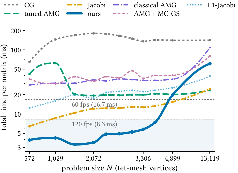
Table Table (also plotted on the figure pages as Fig. 4; per-method runtime breakdown in Supplementary, Table Table) reports per-frame mean solve time and iteration counts. Our method runs at interactive framerates across the full size range: 17.9 ms (\sim\!56 fps, 168 iters) at N\!=\!8\,192 and 47.6 ms (\sim\!21 fps, 394 iters) at N\!=\!16\,384. The closest GPU baseline that converges in the same regime is Jacobi, at 39.5/65.7 ms (968/1543 iters) respectively — \sim\!6\times fewer iterations at N\!=\!8\,192 (968 vs. 168) and \sim\!4\times at N\!=\!16\,384 (1543 vs. 394) on identical hardware, and a 1.42.2\!\times wall-clock gap. Neural SPAI (Yang et al. 2025), re-trained per scale with its CUDA apply path, lands at 48.1/70.9 ms (338/496 iters), trailing our method by 2.7\times at N\!=\!8\,192 and 1.5\times at N\!=\!16\,384 despite an iteration count within \sim\!2\times of ours — the gap is dominated by the two random-gather SpMVs its apply dispatches per iteration, in contrast to our single batched-GEMM apply on contiguous tensors (§5). The IC- and AMG-class baselines reach very low iteration counts (140) but pay for it in sequential triangular solves or V-cycle synchronization, falling below 25 fps at N\!=\!16\,384 — confirming the architectural argument of Table 1. The measured curve is not perfectly linear in N because kernels cross warp/tile-quantization and cache-transition thresholds as the working set grows, even though the algorithmic order remains \Theta(N).

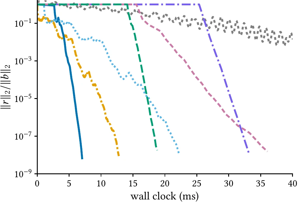
Fig. 5 traces how convergence actually looks on a challenging frame — a closed cross-shaped barrier with stiff density contrast chosen to maximize long-range coupling — across unpreconditioned CG, Jacobi, IC, AMG, and ours, with the right-hand side supported only on thin density interfaces. By k\!=\!1, Jacobi and IC have damped the residual only locally around \mathrm{supp}(b), while AMG and ours have already attenuated it across the whole domain — the visual signature of multiscale transport that the highway buffers implement (§4.3). AMG matches the spread but pays in V-cycle synchronization per iteration; ours runs the inner loop as a single CUDA-Graph capture. Iteration counts on this frame (288/1097/334/19/384 for unprec/Jacobi/IC/AMG/ours) span nearly two orders of magnitude, but per-iteration cost reverses the ranking for AMG and IC. Standard deviations across the 20 test frames track condition number rather than N: Jacobi and unprec. CG show \sigma/\mu\!\approx\!50100\% at N\!\ge\!8\,192 across the [5,100] contrast range, while ours stays at \le\!21\% even at N\!=\!16\,384.

Training dynamics and ablations

Training dynamics and loss.

Fig. 3 tracks \mathcal{L}_{\cos}, the SAI loss on the same checkpoints, and PCG iteration count across training. The three curves move together until step \sim\!8\,000, after which the SAI loss rises from \sim\!10^{-3} to \sim\!0.5 while \mathcal{L}_{\cos} keeps falling in lockstep with PCG iterations — direct evidence of Prop. 1: the model is moving the eigenvalues of MA away from \|A\| in pointwise terms while tightening the relative cluster wherever angular alignment is easiest. Fig. 1 confirms this on the spectrum at N\!=\!1\,024: SAI delivers a 16\times \kappa reduction with the cluster anchored near \|A\|, the same architecture trained with \mathcal{L}_{\cos} delivers 68\times with the cluster wherever it pleased — a 4.3\times gap attributable to the loss alone. Total wall-clock training is 16.2 min on a single H200 (24\,300 steps); the model overtakes GPU Jacobi by step \sim\!2\,000 (\sim\!1.3 min) and drops below 200 PCG iterations by step \sim\!12\,000 (Fig. 6 corroborates the link from probe-space alignment to spectral clustering).

Architecture ablations.

Width d, depth n_l, and highway connections each move total solve time non-trivially. Default (d\!=\!128, n_l\!=\!3, hw on, \sim\!2.6M parameters): (i) shrinking depth n_l\!=\!3\!\to\!1 cuts inference 2.6\times but doubles total solve time because iterations rise 2.5\times (additional layers are needed to compose information routed through the highway tokens); (ii) removing highways raises PCG iterations 2.3\times at N\!=\!2\,048 and the penalty grows with N; (iii) d\!=\!64 is 28\% slower overall, d\!=\!256 is competitive at small N but raises mean PCG iterations from 105 to 191 when averaged over N\!\in\!\{2048,4096,8192\}. Table 4 summarizes the core sweep results; full rows remain in Supplementary, Table Table.

Core architecture ablations (subset of Supplementary Table Table).
Group Configuration Infer. (ms) Iters Total (ms)
Width (avg. N\!\in\!\{2048,4096,8192\}) d{=}64,\;n_l{=}3, hw 3.0 147 15.4
Width (avg. N\!\in\!\{2048,4096,8192\}) d{=}128,\;n_l{=}3, hw 3.1 105 12.0
Width (avg. N\!\in\!\{2048,4096,8192\}) d{=}256,\;n_l{=}3, hw 3.2 191 19.3
Depth (N\!=\!8\,192) d{=}128,\;n_l{=}1, hw 1.3 421 36.9
Depth (N\!=\!8\,192) d{=}128,\;n_l{=}3, hw 3.4 168 17.9
Highways (N\!=\!2\,048) d{=}128,\;n_l{=}3, hw 3.3 66 8.8
Highways (N\!=\!2\,048) d{=}128,\;n_l{=}3, no-hw 2.2 149 13.8

Generalization and what the loss buys

We probe within-family deployment robustness at N\!=\!4\,096 across three shifts — topology (closed barriers withheld from training), contrast (train on \rho_{\text{heavy}}\!\in\![5,25], evaluate on (25,100]), and their composition — and compare three systems on identical eval sets: ours, the same architecture trained instead with the SAI loss of (Yang et al. 2025), and neural SPAI (Yang et al. 2025) trained/evaluated under the same split protocol (Table Table). The same-architecture row is a clean loss ablation; the neural SPAI row is a matched-split learned baseline rather than a full-train upper bound.

Eval distributionmsitersspeedupitersspeedupitersspeedup
Full / in-distribution29.4823.4\times4050.9\times2360.9\times
Closed barriers only24.7683.3\times2081.3\times2580.7\times
High contrast24.41421.9\times1751.5\times2640.7\times
Closed + high contrast25.11471.9\times1741.6\times3960.5\times

Three observations carry the section. (i) Topology generalization is essentially free: withholding closed barriers from training leaves iteration counts unchanged (68 vs. 82), because the \mathcal{H}-matrix partition is keyed to spatial indexing, not barrier geometry. (ii) The loss, not the architecture or the data, is what unlocks the quality. Replacing only the loss — same network, same training distribution — raises iteration counts \sim\!5\times at the in-distribution eval cell (82\!\to\!405); the SAI gradient pins eigenvalues near \|A\|, wasting capacity on a constraint PCG does not care about (Prop. 1). Under matched-split training, neural SPAI sits at 236264 iterations on the first three rows and degrades to 396 on the compositional row. Relative to Jacobi, our row stays at 1.93.4\times speedup across all eval cells, while neural SPAI is 0.9\times, 0.7\times, 0.7\times, and 0.5\times (slower than Jacobi in three of four rows, and substantially slower in the compositional case); the same-architecture SAI ablation reaches only 0.91.6\times. (iii) Contrast is the dominant remaining OOD axis for our method. Pure amplitude growth is absorbed for free by \mathcal{L}_{\cos}’s scale invariance, but far-field interactions at high contrast push the spectrum past the cluster the network has seen — iteration count roughly doubles (82\!\to\!142147) and \sigma/\mu grows fivefold. Full robustness grid in Supplementary, Table Table.

Discussion and Future Work

The recipe — a weak-admissibility \mathcal{H}-matrix prior, a scale-invariant cosine-Hutchinson objective, and a single-graph apply path — is most useful where it targets: stiff, every-frame-different SPD systems with a hard real-time budget. The architecture itself depends on nothing fluid-specific, only a loose spatial ordering of degrees of freedom, and extends directly to 3D (Fig. [fig:teaser]). We expect the largest gains to persist on other SPD families with (i) geometric locality, (ii) frame-to-frame coefficient changes, and (iii) hard real-time budgets (implicit viscosity/diffusion, soft-body and contact dynamics) and smaller gains where a single matrix is reused long enough for heavy classical setup to amortize. Two known limitations are worth flagging: (a) training pre-sizes the partition to a maximum N, so pushing past it currently requires retraining — a dynamic-partition variant (constant leaf count at O(N\log N) rather than constant leaf size at \Theta(N), §4.2) removes this ceiling at the cost of one extra pooling pass per layer; (b) the \mathcal{H}-matrix prior assumes some spatial locality of A under its indexing, and degrades on operators without a natural spatial coordinate (power-grid Laplacians, social-network matrices) or where the far-field rank does not decay with separation.

Fig. 2. Spectra of MA at N\!=\!1\,024 on a representative multiphase Poisson frame (full eigendecomposition; y jittered). Top: unpreconditioned (left) and Jacobi (right). Bottom: same architecture trained with SAI (left, 16\!\times \kappa reduction, cluster anchored near \lambda\!=\!\|A\| as the Frobenius objective demands) versus cosine-Hutchinson (right, 68\!\times reduction, cluster wherever angular alignment is easiest). The 4.3\times gap is attributable entirely to the loss. The bimodal structure in both neural preconditioners reflects the two-phase density contrast of the benchmark.
Fig. 3. Off-diagonal rank audit: provided vs. required. Red: the architecture-provided rank fraction L_s/(SL) at fixed L_s\!=\!32, plotted against off-diagonal distance class S. Dashed: the mean numerical rank fraction required for truncated-SVD approximations of A^{-1} tiles to satisfy \|X-X_r\|_F/\|X\|_F\!\le\!\varepsilon at \varepsilon\!\in\!\{10^{-3},10^{-6},10^{-9}\}, with bands giving \pm 1\sigma over tiles in the same distance class. Required rank drops monotonically with S (far interactions are more compressible) while the architecture’s fixed rank stays above it everywhere, with \sim\!2.6\times headroom in the largest-distance class even at \varepsilon\!=\!10^{-9} — the structural evidence that one shared off-diagonal rank covers every far-field tile (justifying \text{c1}, §4.2).
Fig. 4. Training profile at N\!=\!8\,192 (default config, d\!=\!128, n_l\!=\!3, highways on). Blue: cosine-Hutchinson loss \mathcal{L}_{\cos} (mean \pm 1\sigma over last 100 steps, linear axis). Green dashed: SAI loss (Yang et al. 2025) on a held-out frame at the same checkpoints (log axis); the down-then-up trajectory is the empirical signature of the loss-ablation argument in §7.3 — the model keeps reducing the cosine objective and the PCG iteration count after the SAI surrogate has bottomed out and started to climb. Orange: PCG iterations to \mathrm{rtol}\!=\!10^{-8} on that frame (log). Bottom axis: wall-clock minutes; top axis: optimizer steps. Grey: unpreconditioned CG and Jacobi baselines.
Fig. 5. End-to-end PCG solve time on the multiphase Poisson benchmark across five problem sizes, 20 frames per scale (mean \pm 1\sigma band; relative residual tolerance 10^{-8}). Dashed grey lines mark the 24 and 60 fps interactive budgets. Ours covers \sim\!143 down to \sim\!21 fps; the closest classical GPU baseline (Jacobi) covers \sim\!79 down to \sim\!15 fps; the closest learned baseline (neural SPAI (Yang et al. 2025), re-trained per scale on our benchmark with its CUDA apply path) covers \sim\!54 down to \sim\!14 fps. AMGX SPAI and GPU IC sit above 40 ms across all scales despite much lower iteration counts, dominated by unparallelizable triangular solves or V-cycle synchronization. Full per-method times and iteration counts appear in Table Table.
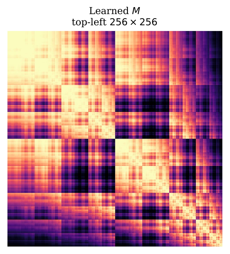
Fig. 6. Multiscale error transport across preconditioner families on a challenging multiphase Poisson frame (closed cross-barrier topology, stiff density contrast), distinct from the teaser frame. Top row: density \rho, right-hand side b, pressure p, |v|, and a top-left view of the learned M. Rows below, top to bottom: unpreconditioned CG, Jacobi, IC, AMG, ours. Each row shows |r_k| on a shared log color scale at five iteration snapshots; row labels give each method’s iteration count to \mathrm{rtol}\!=\!10^{-8}. At k\!=\!1, Jacobi and IC damp error only locally around \mathrm{supp}(b), while AMG and ours have already attenuated the residual across the whole domain — direct evidence that the learned M routes correction signals across graph-distant regions in a single apply, the global routing pattern the highway buffers implement (§4.3). AMG matches the spread but pays in V-cycle synchronization per iteration; ours runs the inner loop as a single CUDA-Graph-captured sequence of batched GEMMs (§5).
Fig. 7. Probe-alignment dynamics during training at N\!=\!8\,192 (d\!=\!128, n_l\!=\!3, highways on), over checkpoints in the 8k–24k step range. Each probe (point) is plotted by the angle its image MA\mathbf{z} makes with \mathbf{z} in \mathbb{R}^N, early in training (left) vs. late (right). As \mathcal{L}_{\cos} drives the per-probe angle to zero, the point cloud collapses inward — the spatial signature of the spectral clustering of MA that Fig. 1 shows at N\!=\!1\,024 and that Fig. 3 shows in PCG iteration counts.
Benzi, Michele, Carl D. Meyer, and Miroslav Tŭma. 1996. “A Sparse Approximate Inverse Preconditioner for the Conjugate Gradient Method.” SIAM Journal on Scientific Computing 17 (5): 1135–49.
Börm, Steffen, Lars Grasedyck, and Wolfgang Hackbusch. 2003. Introduction to Hierarchical Matrices with Applications. Engineering Analysis with Boundary Elements.
Chen, Jie. 2024. “Graph Neural Preconditioners for Iterative Solutions of Sparse Linear Systems.” arXiv Preprint arXiv:2406.00809. https://arxiv.org/abs/2406.00809.
Fan, Yuwei, Lin Lin, Lexing Ying, and Leonardo Zepeda-Núñez. 2019. “A Multiscale Neural Network Based on Hierarchical Matrices.” arXiv Preprint arXiv:1807.01883. https://arxiv.org/abs/1807.01883.
Fognini, Emilio McAllister, Marta M. Betcke, and Ben T. Cox. 2025. “Learning Green’s Operators Through Hierarchical Neural Networks Inspired by the Fast Multipole Method.” arXiv Preprint arXiv:2509.20591. https://arxiv.org/abs/2509.20591.
Greengard, Leslie, and Vladimir Rokhlin. 1987. “A Fast Algorithm for Particle Simulations.” Journal of Computational Physics 73 (2): 325–48. https://doi.org/10.1016/0021-9991(87)90140-9.
Hackbusch, Wolfgang. 1999. A Sparse Matrix Arithmetic Based on \mathcal{H}-Matrices. Part I: Introduction to \mathcal{H}-Matrices. Berlin: Springer.
Hackbusch, Wolfgang, and Boris N. Khoromskij. 2002. Adaptive \mathcal{H}-Matrix Approximation on General Domains. Springer.
Hartland, Tucker, Georg Stadler, Mauro Perego, Kim Liegeois, and Noémi Petra. 2023. “Hierarchical Off-Diagonal Low-Rank Approximation of Hessians in Inverse Problems, with Application to Ice Sheet Model Initialization.” arXiv Preprint arXiv:2301.03644. https://arxiv.org/abs/2301.03644.
Häusner, Paul, Ozan Öktem, and Jens Sjölund. 2023. “Neural Incomplete Factorization: Learning Preconditioners for the Conjugate Gradient Method.” arXiv Preprint arXiv:2305.16368. https://arxiv.org/abs/2305.16368.
Hutchinson, Michael F. 1989. “A Stochastic Estimator of the Trace of the Influence Matrix for Laplacian Smoothing Splines.” Communications in Statistics—Simulation and Computation 18 (3): 1059–76.
Ihmsen, Markus, Nadir Akinci, Markus Becker, and Matthias Teschner. 2011. “A Parallel SPH Implementation on Multi-Core CPUs.” Computer Graphics Forum 30 (1): 99–112.
Karras, Tero. 2012. “Maximizing Parallelism in the Construction of BVHs, Octrees, and k-d Trees.” In Proc. ACM SIGGRAPH/Eurographics Conf. On High-Performance Graphics (HPG), 33–37.
Kipf, Thomas N., and Max Welling. 2017. “Semi-Supervised Classification with Graph Convolutional Networks.” In International Conference on Learning Representations (ICLR).
Kolotilina, L. Yu., and A. Yu. Yeremin. 1993. “Factorized Sparse Approximate Inverse Preconditionings I: Theory.” SIAM Journal on Matrix Analysis and Applications 14 (1): 45–58.
Li, Yichen, Peter Yichen Chen, Tao Du, and Wojciech Matusik. 2023. “Learning Preconditioners for Conjugate Gradient PDE Solvers.” arXiv Preprint arXiv:2305.16432. https://arxiv.org/abs/2305.16432.
Li, Zongyi, Nikola Kovachki, Kamyar Azizzadenesheli, Burigede Liu, Kaushik Bhattacharya, Andrew Stuart, and Anima Anandkumar. 2020a. “Multipole Graph Neural Operator for Parametric Partial Differential Equations.” Advances in Neural Information Processing Systems 33.
———. 2020b. “Neural Operator: Graph Kernel Network for Partial Differential Equations.” arXiv Preprint arXiv:2003.03485. https://arxiv.org/abs/2003.03485.
———. 2021. Fourier Neural Operator for Parametric Partial Differential Equations.” In International Conference on Learning Representations. https://openreview.net/forum?id=c8P9NQVtmnO.
Lin, Chih-Jen, and Jorge J. Moré. 1999. “Incomplete Cholesky Factorizations with Limited Memory.” SIAM Journal on Scientific Computing 21 (1): 24–45.
Liu, Lijun, Shengguo Li, Xiangke Hu, Yutong Wang, Xuejun Liu, and Jingling Xue. 2016. “Exploring Data Level Parallelism in Incomplete LU Factorization on GPUs.” IEEE Transactions on Parallel and Distributed Systems 27 (12): 3397–3410.
Liu, Ze, Yutong Lin, Yue Cao, Han Hu, Yixuan Wei, Zheng Zhang, Stephen Lin, and Baining Guo. 2021. Swin Transformer: Hierarchical Vision Transformer Using Shifted Windows.” arXiv Preprint arXiv:2103.14030. https://arxiv.org/abs/2103.14030.
Lu, Lu, Pengzhan Jin, Guofei Pang, Zhongqiang Zhang, and George Em Karniadakis. 2021. “Learning Nonlinear Operators via DeepONet Based on the Universal Approximation Theorem of Operators.” Nature Machine Intelligence 3 (3): 218–29.
Luz, Ilay, Meirav Galun, Haggai Maron, Ronen Basri, and Irad Yavneh. 2020. “Learning Algebraic Multigrid Using Graph Neural Networks.” arXiv Preprint arXiv:2003.05744. https://arxiv.org/abs/2003.05744.
Lyu, Kangbo, Ruihong Cen, Yushen Wu, and Tao Du. 2026. “A Multigrid-Inspired Neural Iterative Solver for Poisson Equations on Large Voxel Grids.” https://openreview.net/forum?id=lNcbGSWhJo.
Naumov, Maxim, Michael Chien, Paul Vandermersch, Ujval Kapasi, Boris Catanzaro, and Michael Garland. 2015. cuSPARSE Library.” In GPU Technology Conference (GTC).
Raissi, Maziar, Paris Perdikaris, and George Em Karniadakis. 2019. “Physics-Informed Neural Networks: A Deep Learning Framework for Solving Forward and Inverse Problems Involving Nonlinear Partial Differential Equations.” Journal of Computational Physics 378: 686–707.
Rudikov, Kirill, Anastasia Markeeva, Vasily Bulatov, and Dmitry Vetrov. 2024. “Neural Functional Operator for Parametric PDEs.” arXiv Preprint arXiv:2402.01030. https://arxiv.org/abs/2402.01030.
Ruge, John W., and Klaus Stüben. 1987. “Algebraic Multigrid (AMG).” Multigrid Methods 3: 73–130.
Saad, Yousef. 2003. Iterative Methods for Sparse Linear Systems. 2nd ed. Philadelphia, PA: SIAM.
Sittoni, Pietro, Emanuele Zangrando, Angelo Alberto Casulli, Nicola Guglielmi, and Francesco Tudisco. 2026. Neural-HSS: Hierarchical Semi-Separable Neural PDE Solver.” arXiv Preprint arXiv:2602.18248. https://arxiv.org/abs/2602.18248.
Teschner, Matthias, Bruno Heidelberger, Matthias Müller, Danat Pomerantes, and Markus H. Gross. 2003. “Optimized Spatial Hashing for Collision Detection of Deformable Objects.” In Vision, Modeling, and Visualization (VMV), 47–54.
Trifonov, Vladislav, Ekaterina Muravleva, and Ivan Oseledets. 2025. “Message-Passing GNNs Fail to Approximate Sparse Triangular Factorizations.” arXiv Preprint arXiv:2502.01397. https://arxiv.org/abs/2502.01397.
Trifonov, Vladislav, Alexander Rudikov, Oleg Iliev, Yuri M. Laevsky, Ivan Oseledets, and Ekaterina Muravleva. 2024. “Learning from Linear Algebra: A Graph Neural Network Approach to Preconditioner Design for Conjugate Gradient Solvers.” arXiv Preprint arXiv:2405.15557. https://arxiv.org/abs/2405.15557.
Vaswani, Ashish, Noam Shazeer, Niki Parmar, Jakob Uszkoreit, Llion Jones, Aidan N. Gomez, Łukasz Kaiser, and Illia Polosukhin. 2017. “Attention Is All You Need.” In Advances in Neural Information Processing Systems 30 (NIPS 2017), 5998–6008.
Wu, Felix, Amauri Souza, Tianyi Zhang, Christopher Fifty, Tao Yu, and Kilian Weinberger. 2019. “Simplifying Graph Convolutional Networks.” In Proceedings of the 36th International Conference on Machine Learning, 97:6861–71. Proceedings of Machine Learning Research. PMLR. http://proceedings.mlr.press/v97/wu19e.html.
Xu, Tianshi, Rui Peng Li, and Yuanzhe Xi. 2025. “Neural Approximate Inverse Preconditioners.” arXiv Preprint arXiv:2510.13034. https://arxiv.org/abs/2510.13034.
Yamazaki, Ichitaro, Stanimire Tomov, and Jack Dongarra. 2020. “Mixed-Precision Cholesky QR Factorization and Its Parallelization on GPUs.” Parallel Computing 99: 102693.
Yang, Zherui, Zhehao Li, Kangbo Lyu, Yixuan Li, Tao Du, and Ligang Liu. 2025. “Learning Sparse Approximate Inverse Preconditioners for Conjugate Gradient Solvers on GPUs.” arXiv Preprint arXiv:2510.27517. https://arxiv.org/abs/2510.27517.

Supplementary Material