Rigid Origami Solver

A high-performance rigid-body solver for origami patterns: faces are treated as rigid plates connected by rotational hinges, and the system is solved as a constrained kinematic network rather than a mass-spring model.

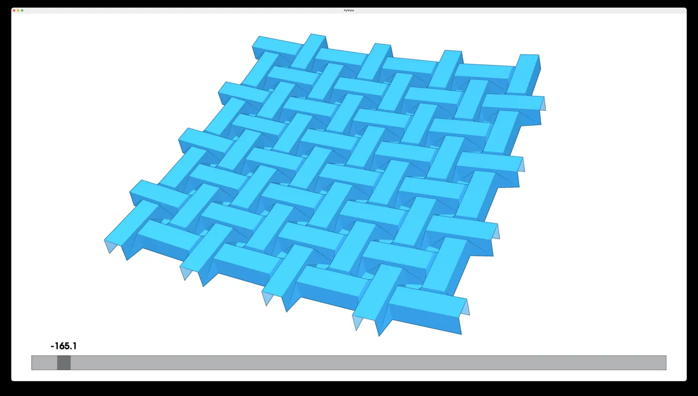
Simulated Huffman rectangular-weave pattern solved for geometric closure.

How it works

The state of the sheet is the vector of dihedral fold angles. For every internal vertex, the product of edge-frame rotations around that vertex must equal the identity — that's the rigid-foldability closure constraint.

Governing equations

For a vertex with $k$ incident edges:

$$R_z(\alpha_1) R_x(\rho_1) \cdots R_z(\alpha_k) R_x(\rho_k) - I_3 = 0$$

Splitting fold angles into free unknowns $x$ and user-driven inputs $u$ , with static sector angles $\alpha$ and connectivity $p$ as parameters, the constraints become a residual $f(x, p, u) = 0$ solved by root-finding.

Damped Newton with trust region

Plain Newton fails at the flat sheet: the configuration is singular, the Jacobian goes rank-deficient, and the solver flips between mountain and valley assignments (bifurcation). The solver instead uses a step-limited damping scheme that constrains each iteration to the local basin of attraction, preserving the mountain/valley pattern across frames.

The linear sub-problem $J \Delta x = -F(x)$ is solved with scipy.sparse.linalg.lsmr, chosen over LSQR for monotonic convergence on the rank-deficient cases near bifurcation points.

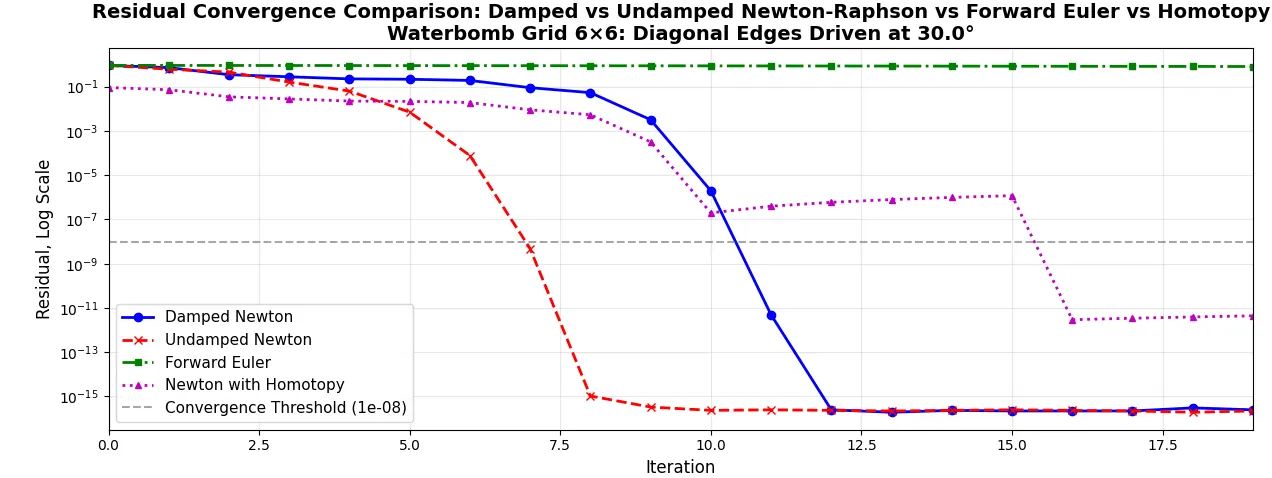
Forward Euler fails to converge; undamped Newton bifurcates; damped Newton stays in the local basin.

Sparse analytical Jacobian

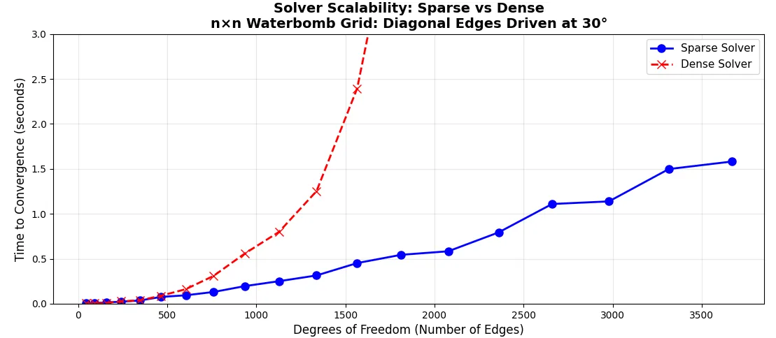
Closure constraints are topologically local — each fold only affects vertices it touches — so the Jacobian is over 98% sparse on large grids. The solver:

• Computes analytical derivatives via the chain rule on $SO(3)$ (no finite differences).
• Assembles entries directly into pre-allocated flat COO arrays.
• Parallelizes assembly with Numba prange, bypassing the GIL.

Beyond ~200 DOFs the dense solver hits an $O(N^3)$ wall; the sparse solver scales empirically as ≈ $O(N^{1.2})$ and stays interactive on a 70×70 Miura grid.

Visualization

3D coordinates are reconstructed from fold angles in $O(N)$ by a BFS over the face graph rooted at the center, propagating rigid transforms via Rodrigues' formula. PyVista handles the live rendering.

Patterns

The repository includes .fold files for:

• birdBase.fold, flappingBird.fold — classical Miura-derived bases
• huffmanWaterbomb.fold, huffmanRectangularWeave.fold, huffmanExdentedBoxes.fold — Huffman tessellations

Non-rigid patterns (e.g. flapping bird, which physically requires panel bending) correctly stagnate at a non-zero residual: no rigid configuration exists, and the solver reports it rather than producing spurious motion.

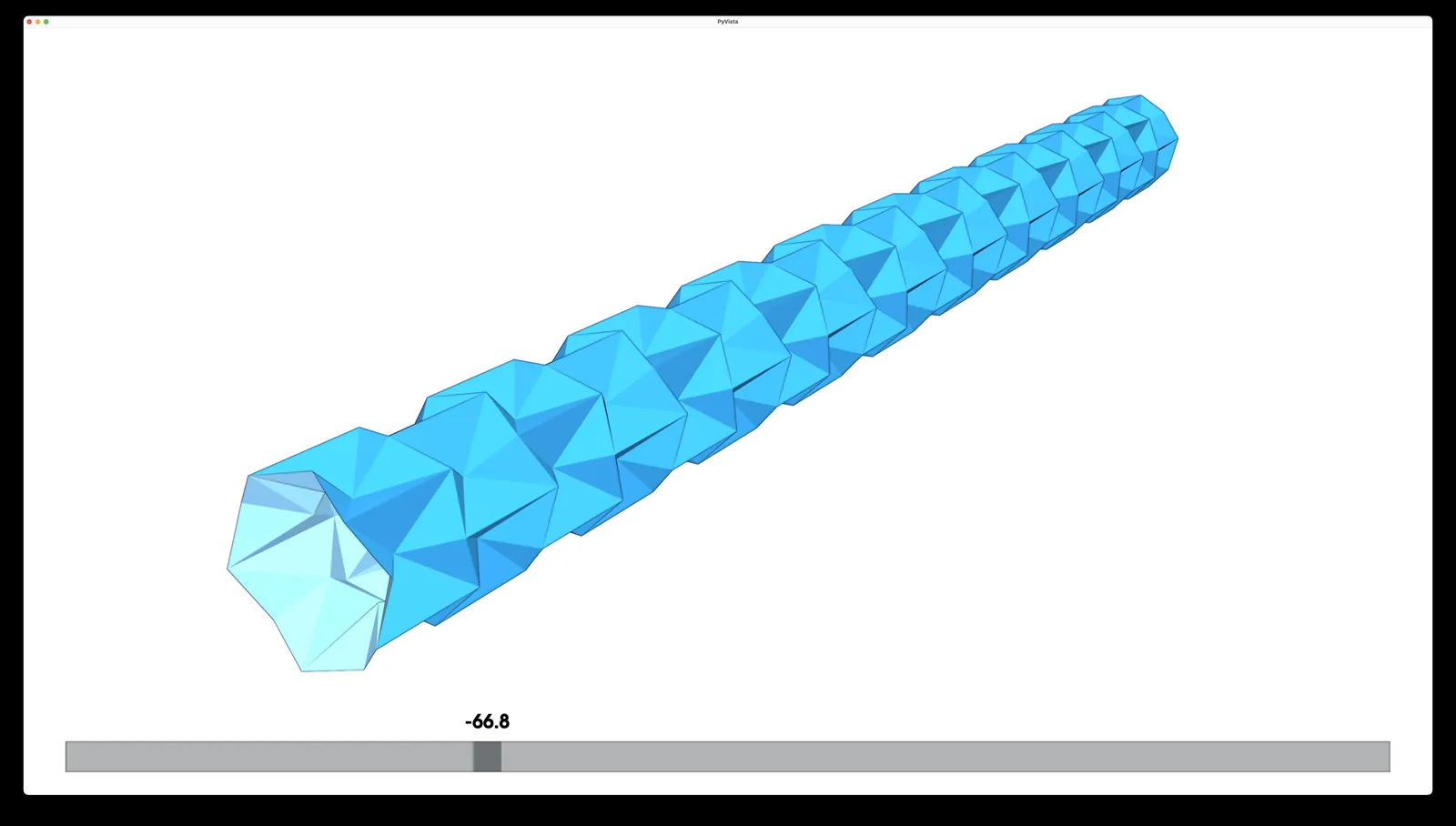
Additional results

Stack

• Python — NumPy, SciPy (lsmr), Numba (JIT + prange)
• PyVista — interactive 3D visualization

License

MIT — see LICENSE.